


Mental health monitoring among schoolchildren
The study encompasses 89 counties in Jiangsu Province, China (Fig. 1, Fig. S1). Daily records detailing children’s absences due to mental distress were sourced from the national school health monitoring system, collaboratively managed by educational institutions and regional disease control centers23. The reporting procedure involves the child’s guardian or class teacher initially filling out a questionnaire to report symptoms to the school doctor or community hospital. These health professionals then confirm the mental health diagnosis and document the absence’s specifics, including duration (start and end dates), type of mental health condition, symptoms presented, individual characteristics, and contextual information from the school and region. This comprehensive documentation process also includes collecting oral symptom descriptions from parents and details of any related outpatient or hospitalization. For absences following hospital visits, medical documentation must be provided to the school, ensuring informed consent for the child’s return to class. Quality control of data collection is conducted daily by staff at the regional disease control center (Text S1).

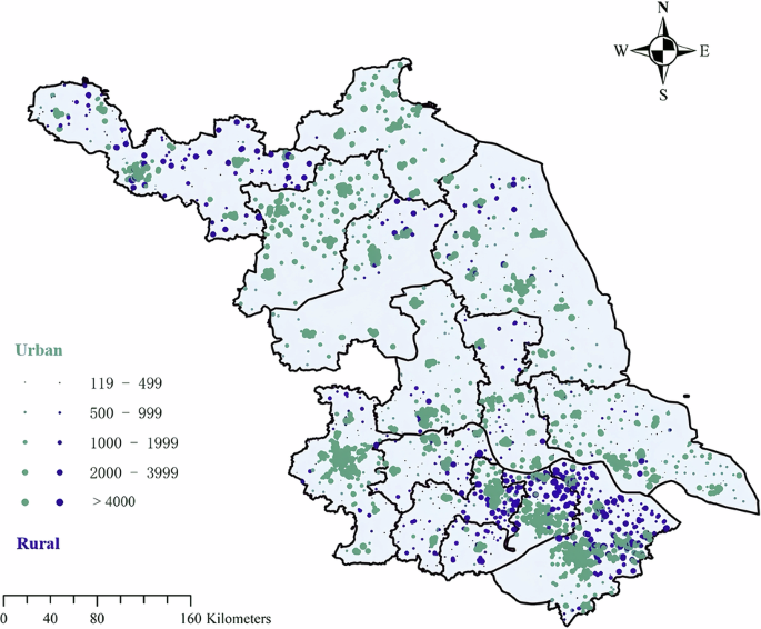
Spatial distribution of urban and rural schools across 89 counties in Jiangsu Province, China.
During the data cleaning process, mental health diseases and symptoms were extracted according to the International Statistical Classification of Diseases and Related Health Problems, 10th Revision (ICD-10), including disorders such as depression, neurasthenia, and anxiety. To mitigate confounding effects, several measures were implemented: (1) potential mental discomfort related to academic stress, other diseases, or physical injuries was controlled based on the text recognition of corpus; (2) COVID-19-related records, including children with COVID-19 or had intersecting activity paths with COVID-19 cases, were excluded; (3) Given the limited and inconsistent evidence linking air pollution to severe mental disorders, especially in children, and the influence of multiple other risk factors such as genetics and family environment14,24,25,26, this study focused on short-term exposure effects and excluded absences lasting 1 week or longer to better capture environmentally induced acute responses; (4) for individuals with multiple consecutive absences, only the initial date of the absence period was retained to minimize confounding from repeated events. The geographic coordinates (longitude and latitude) of each school were matched by the geographic information system using a unique identification code for the region and the school. Data extraction, collection, and quality control were facilitated by the Jiangsu Provincial Center for Disease Control and Prevention. The final dataset comprises 95,658 records of personal absences due to mental health issues from 2016 to 2021 across primary and secondary schools. From these records, we derived a multi-school-centered time series dataset summarizing daily counts and rates of mental distress-related absences. Detailed data cleaning procedures and the keywords for identifying mental distress are documented in Text S1, S2.
Overall, the study was based on de-identified data obtained from the Jiangsu Center for Disease Control and Prevention, with no direct participant contact, identifiable information, or collection of biological specimens involved. Data use was authorized for research purposes in accordance with the Declaration of Helsinki.
Particulate matter and non-optimal temperature exposure estimation
High-resolution daily estimates of particulate matter concentrations, including PM1, PM2.5, and PM10, were obtained from the China High Air Pollutants (CHAP) dataset for the period 2016 to 2021, with a spatial resolution of 1 km27,28,29. These exposure data were derived from Moderate Resolution Imaging Spectroradiometer (MODIS) Multi-Angle implementation of Atmospheric Correction (MAIAC) aerosol products using developed spatiotemporal machine learning models. The cross-validation coefficients of determination (CV-R2) for PM1, PM2.5, and PM10 were reported as 0.83, 0.92, and 0.90, respectively27,28,30. Using the k-nearest neighbors (k-NN) algorithm implemented in the FNN package in R version 3.6.1, we quantified the daily pollution exposure for each school over the previous 0–14 days. This non-parametric algorithm is favored for its straightforward implementation and effectiveness in handling complex relationships between features and outcomes that are not readily modeled by parametric approaches31. It operates by identifying the nearest particulate matter grid center points to each school location based on geographic proximity, thereby accurately estimating localized environmental exposure. The average ambient concentrations of ambient particulate matter in school environment were 23 µg/m³ for PM1, 38 µg/m³ for PM2.5, and 70 µg/m³ for PM10.
Hourly temperature simulation (2-meter temperature index) at a resolution of 9-km was derived from the ERA5-Land meteorological reanalysis dataset, provided by the European Centre for Medium-Range Weather Forecasts32. We also derived daily average temperature (DAT) in the past 0–14 days based on 24-h temperature for each school through k-NN algorithm. Moreover, we calculated the accordingly intra-day change (IDC) of temperature derived from max and min hour temperature on the day, as well as IDFs based on the DAT between the lag day and the lag previous day9.
Co-exposure assessment
Compound environmental exposure scenarios were constructed by first identifying threshold values, then combining averaged 14-day PM concentrations with non-optimal temperatures based on established benchmarks, and finally applying gender-specific stratification.
First, for particulate matter, PM2.5 and PM10 were categorized according to China national Grade I Ambient Air Quality Standards (GB 3095-2012)33,34, which define 24-h average concentration limits of 35 µg/m³ and 50 µg/m³, respectively. In contrast, no official standard exists for PM1. Therefore, a concentration of 22 µg/m3, the median value observed across the study period, was adopted as a threshold to define low and high exposure categories. This choice was based on previous studies that used the median as a PM cutoff in the absence of a regulatory benchmark or in the desire to focus on relative high-low pollution35,36,37, which also ensured balanced group sizes and accounted for local pollution patterns. Although the World Health Organization’s 24-h guideline value for PM2.5 (15 µg/m3) is considered a more generalizable threshold, it was ultimately excluded from stratified analyses because nearly all measurements across the study locations exceeded this value. This limitation is addressed in the discussion. Consequently, PM1, PM2.5, and PM10 were classified into low- and high-exposure categories at thresholds of 22 µg/m³, 35 µg/m³, and 50 µg/m³, respectively.
Regarding ambient temperature, no universal standard defines thermally optimal conditions across different climates or health outcomes38,39. We therefore adopted an epidemiological approach based on the concept of non-optimal temperature exposure40. Non-optimal temperature refers to any ambient temperature that is either higher or lower than the theoretical minimum risk exposure level, which is defined as the temperature associated with the lowest overall health risk for a given location. Specifically, risk thresholds were determined by identifying the minimum-risk temperature using exposure–response curves derived from single-exposure models of temperature related absenteeism. Considering the risk thresholds derived from our single temperature exposure models, we developed specific criteria for categorizing temperature exposure. A threshold of 10 °C was used to differentiate between suitable and unsuitable temperature conditions for DAT and IDC. IDF was further segmented into cooling, suitable, and warming categories, using −2.5 °C and 0 °C as cut-offs. These classifications enable the analysis of the compound impacts of air pollution and temperature variability on health outcomes.
Then, we devised nine composite exposure scenarios by integrating PM1, PM2.5 and PM10 with DAT, IDC and IDF including DAT-PM (DAT-PM1, DAT-PM2.5, DAT-PM10), IDC-PM (IDC-PM1, IDC-PM2.5, IDC-PM10), and IDF-PM (IDF-PM1, IDF-PM2.5, IDF-PM10). These scenarios are structured into differentiated levels based on the combinations of particulate matter and temperature conditions. Specifically, DAT-PM1-10 had 4 levels, including (1) Suitable DAT and low-level PM (level 1); (2) Suitable DAT and high-level PM (level 2); (3) Unsuitable DAT and low-level PM (level 3); and (4) Unsuitable DAT and high-level PM (level 4); IDC-PM1-10 had 4 levels, including (1) Suitable IDC and low-level PM (level 1); (2) Suitable IDC and high-level PM (level 2); (3) Unsuitable IDC and low-level PM (level 3); and (4) Unsuitable IDC and high-level PM (level 4); IDF-PM1-10 had 6 levels, including (1) Suitable IDF and low-level PM (level 1); (2) Suitable IDF and high-level PM (level 2); (3) Cooling IDF and low-level PM (level 3); and (4) Cooling IDF and high-level PM (level 4); (5) Warming IDF and low-level PM (level 3); and (4) Warming IDF and high-level PM (level 6). For all scenarios, Level 1 is designated as the reference group against which all other levels are compared.
Finally, to explore potential gender differences in co-exposure scenarios, we refined the composite exposure indicators into binary variables, where ‘0’ denotes non-composite exposure days, including scenarios of low pollution with suitable temperatures, low pollution with unsuitable temperatures, and high pollution with suitable temperatures; “1” indicates days of identified co-exposure characterized by high pollution with unsuitable temperature conditions. Building on this framework, we integrated gender-specific co-exposure indicators to conduct interaction term tests and subgroup analyses, aiming to assess the differential resilience to environmental stressors between males and females (0–0: males in no co-exposure days, 0–1: females in no co-exposure days, 1–0: males in co-exposure days, and 1–1: females in co-exposure days). Please refer to Fig. S2 for the flowchart of composite indicator construction.
Covariates
We calculated the daily relative humidity (RH) over the past 14 days using air pressure, dew point temperature, and surface temperature data obtained from the ERA5-Land meteorological reanalysis dataset32. Other variables covered included year, season, day of the week (DOW), region (urban and rural), gender, grade, medical symptoms, diagnostic causes, medical choice (outpatient, hospitalization, at home), start and end dates of absenteeism, and school enrollment were considered by subgroup analysis or as controls to mitigate potential spatial and temporal confounding factors.
Statistical analysis
We employed a space-time stratified design that integrates quasi-binomial regression models with distributed lag linear and non-linear functions to examine the associations between air pollution, non-optimal temperatures, and the incidence of mental distress among school-aged children41. This design adjusts for overdispersion in absenteeism rate42, and controls for spatial and temporal variations at the school level, accounting for regional and school-specific environmental factors that are constant within the time window. Based on the characteristics of school time-series statistics, the stratum is defined as a categorical variable of the school-specific year and DOW (e.g., school code-year-DOW). This stratification helps address potential confounding factors such as long-term trends, short-term holiday effects, and inter-school variations. The model is specified as follows:
$${\rm{logit}}(p)=\alpha +{\beta }_{0}* {\rm{exposure}}+{\beta }_{1}* {\rm{stratum}}+{\beta }^{{\rm{T}}}* {\rm{covariates}}$$
(1)
Where p represents the daily absenteeism rate due to mental distress, α is the intercept, exposure includes particulate matter or non-optimal temperature treated with cross-basis functions with coefficient β0, stratum adjusts for location-specific temporal window, and covariates are additional confounders with coefficients βT.
For particulate matter, we applied a linear trend using a one-basis matrix in accordance with the previous findings demonstrating a positive linear relationship43,44, while for non-optimal temperatures, we used a natural cubic spline to capture non-linear effects45. When taking the single exposure model, additional external exposure factors were considered as confounders. To account for the influence of RH, a natural cubic spline with three degrees of freedom was utilized. Furthermore, we modeled both lagged and cumulative effects for exposures ranging from 0 to 14 days. The relative risk associated with a 10 μg/m³ increase in particulate matter exposure, along with the corresponding 95% confidence interval (95% CI), was calculated to quantify the potential impact on mental health.
We conducted Pearson correlation analysis and k-means cluster analysis to explore the relationships between PM exposure and temperature environments. Structural equation modeling (SEM) was employed to investigate the path dependencies of PM and temperatures on school absenteeism using daily county-level records. The analysis was performed using the lavaan package in R version 3.6.1. The latent variable PM was defined by three observed indicators (PM1, PM2.5, and PM10). Structural models were estimated with school absenteeism regressed on PM, DAT, IDC, and IDF using the sem function. Model fit was assessed through comprehensive summary statistics and fit indices obtained using the summary and fitMeasures functions. Additionally, path diagrams were generated using the lavaanPlot function, displaying standardized estimates and significance levels.
To evaluate the compound effects on children’s mental distress–related absenteeism, we first dichotomized the absenteeism rate based on its median, defining a binary outcome variable. We then employed a conditional logistic regression model with a binomial distribution to assess the interactive effects of various exposure conditions during the past 0–14 days. The reference group was defined as exposure to low PM pollution under suitable temperature conditions. The effects were evaluated using three indicators: the Relative Excess Over Expected Interaction (REOI), the Attributable Proportion due to Interaction (AP), and the Synergy Index (S)46. These metrics represent the interaction effect component, the proportion of the total effect attributable to interaction, and the ratio between the total effect and the individual effects, respectively. The formulas are as follows:
$$\begin{array}{lll}\mathrm{REOI}&=&({{\rm{O}}}_{11}-1)-({\mathrm{OR}}_{10}-1)-({\mathrm{OR}}_{01}-1)\\ &=&{\mathrm{OR}}_{11}-{\mathrm{OR}}_{10}-{\mathrm{OR}}_{01}+1\end{array}$$
(2)
$${\rm{AP}}={\rm{REOI}}/{{\rm{OR}}}_{11}$$
(3)
$${\rm{S}}=({{\rm{OR}}}_{11}-1)/[({{\rm{OR}}}_{10}-1)+({{\rm{OR}}}_{01}-1)]$$
(4)
Where OR represents the odds of mental health related absenteeism under different exposure scenarios relative to the reference group (low pollution-suitable temperature), OR11 represents the odds ratio for the joint exposure to both high PM and non-optimal temperature condition, OR10 for PM exposure alone, and OR01 for non-optimal temperature alone.
Additionally, the interaction term was induced to explore risk differences and trends associated with gender across exposure scenarios. Specifically, we compared the relative risks among males in composite exposure, females in non-composite exposure, and females in composite exposure, with males in a non-composite exposure environment serving as the reference group.
Sensitivity analysis
We tested the risk trends over 0–14 days and weighted the absence period as an alternative metric to the absence rate evaluation index. We conducted stratified analyses to investigate effect modifications across various dimensions, including gender, region, season, specific mental disorders such as neurasthenia and depression, types of educational institutions, and medical choice. Furthermore, the COVID-19 outbreak was incorporated as a time-stratified adjustment within the basic model to evaluate its comprehensive impacts (Fig. S3). We also performed generalized linear regression models based on overall records to ensure the robustness of the exposure-response relationship (Figs. S4, S5, Table S1). In addition, we further examined the robustness of risk associations after adjusting for O3 exposure, as well as the potential risks attributable to O3 under both independent and joint exposure scenarios, to extend the scope of discussion. All analysis was performed by R version 3.6.1 with two-tailed test significance *p < 0.05, **p < 0.01, ***p < 0.001.
link